Python solves the XOR problem

Nonlinear relationship to solve XOR problem

This article explains the use of non-linear neural networks to solve the XOR problem, the method of parameter initialization, and the reason for using crossEntropy instead of MSE in classification problems.

First, the normal solution to the XOR relationship

import numpy as np

import matplotlib.pyplot as plt

x_data = np.array([[1,0,0],

[1,0,1],

[1,1,0],

[1,1,1]])

y_data = np.array([[0],

[1],

[0]])

# Initialize the weight, the value range is -1~1

v = (np.random.random([3,4])-0.5)*2

w = (np.random.random([4,1])-0.5)*2

lr = 0.11

def sigmoid(x):

return 1/(1+np.exp(-x))

def d_sigmoid(x):

return x*(1-x)

def update():

global x_data,y_data,w,v,lr,L1,L2,L2_new

L1 = sigmoid(np.dot(x_data,v)) #The output 4*4 matrix of the hidden layer

L2 = sigmoid(np.dot(L1,w)) #The actual output of the output layer 4*1

# Calculate the error of the output layer and the hidden layer, and then find the update amount

L2_delta = (L2-y_data) # y_data 4*1 matrix

L1_delta = L2_delta.dot(wT)*d_sigmoid(L1)

# Update the weights from the input layer to the hidden layer and the weights from the hidden layer to the output layer

w_c = lr*L1.T.dot(L2_delta)

v_c = lr*x_data.T.dot(L1_delta)

w = w-w_c

v = v-v_c

L2_new = softmax(L2)

def cross_entropy_error(y, t):

return -np.sum(t * np.log(y)+(1-t)*np.log(1-y))

def softmax(x):

exp_x = np.exp(x)

sum_exp_x = np.sum(exp_x)

y = exp_x/sum_exp_x

return y

if __name__=='__main__':

for i in range(1000):

update() #Update weights\

if i%10==0:

plt.scatter(i,np.mean(cross_entropy_error(L2_new,y_data)))

plt.title('error curve')

plt.xlabel('iteration')

plt.ylabel('error')

plt.show()

print(L2)

print(cross_entropy_error(L2_new,y_data))

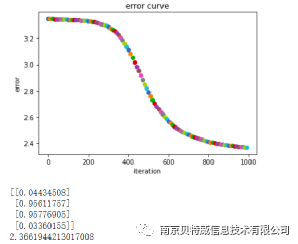
Let's talk about the input data x first: the first column is the bias item is always set to 1, and the last two columns are x1, x2 respectively. And y is the output corresponding to x1, x2, that is, the label of the result of the XOR relationship. lr is the set learning rate. Loss is calculated by cross-entropy. Finally, the prediction result below the figure is obtained, and it is not difficult to see that the prediction result is still very close to the label .

2. Use a linear relationship to solve the XOR problem

import numpy as np

import matplotlib.pyplot as plt

x_data = np.array([[1,0,0],

[1,0,1],

[1,1,0],

[1,1,1]])

y_data = np.array([[0],

[1],

[0]])

# Initialize the weight, the value range is -1~1

v = (np.random.random([3,4])-0.5)*2

w = (np.random.random([4,1])-0.5)*2

lr = 0.11

def update():

global x_data,y_data,w,v,lr,L1,L2,L2_new

L1 = np.dot(x_data,v) #The output 4*4 matrix of the hidden layer

L2 = np.dot(L1,w) #The actual output of the output layer 4*1

# Calculate the error of the output layer and the hidden layer, and then find the update amount

L2_delta = (L2-y_data) # y_data 4*1 matrix

L1_delta = L2_delta.dot(wT)

# Update the weights from the input layer to the hidden layer and the weights from the hidden layer to the output layer

w_c = lr*L1.T.dot(L2_delta)

v_c = lr*x_data.T.dot(L1_delta)

w = w-w_c

v = v-v_c

L2_new = softmax(L2)

def cross_entropy_error(y, t):

return -np.sum(t * np.log(y)+(1-t)*np.log(1-y))

def softmax(x):

exp_x = np.exp(x)

sum_exp_x = np.sum(exp_x)

y = exp_x/sum_exp_x

return y

if __name__=='__main__':

for i in range(300):

update() #update weights

if i%10==0:

plt.scatter(i,np.mean(cross_entropy_error(L2_new,y_data)))

plt.title('error curve')

plt.xlabel('iteration')

plt.ylabel('error')

plt.show()

print(L2)

print("The final error size is: ",cross_entropy_error(L2_new,y_data))

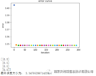
It is not difficult to see that the XOR problem cannot be solved using a linear relationship .

3. Use MSE as a loss function to solve the XOR problem

import numpy as np

import matplotlib.pyplot as plt

x_data = np.array([[1,0,0],

[1,0,1],

[1,1,0],

[1,1,1]])

y_data = np.array([[0],

[1],

[0]])

# Initialize the weight, the value range is -1~1

v = (np.random.random([3,4])-0.5)*2

w = (np.random.random([4,1])-0.5)*2

lr = 0.11

def sigmoid(x):

return 1/(1+np.exp(-x))

def d_sigmoid(x):

return x*(1-x)

def update():

global x_data,y_data,w,v,lr,L1,L2,L2_new

L1 = sigmoid(np.dot(x_data,v)) #The output 4*4 matrix of the hidden layer

L2 = sigmoid(np.dot(L1,w)) #The actual output of the output layer 4*1

L2_delta = (L2-y_data)*d_sigmoid(L2) # y_data 4*1 matrix

L1_delta = L2_delta.dot(wT)*d_sigmoid(L1)

# Update the weights from the input layer to the hidden layer and the weights from the hidden layer to the output layer

w_c = lr*L1.T.dot(L2_delta)

v_c = lr*x_data.T.dot(L1_delta)

w = w-w_c

v = v-v_c

L2_new = softmax(L2)

def softmax(x):

exp_x = np.exp(x)

sum_exp_x = np.sum(exp_x)

y = exp_x/sum_exp_x

return y

if __name__=='__main__':

for i in range(1000):

update() #Update weights\

if i%10==0:

plt.scatter(i,np.mean((y_data-L2)**2)/2)

plt.title('error curve')

plt.xlabel('iteration')

plt.ylabel('error')

plt.show()

print(L2)

print(np.mean(((y_data-L2)**2)/2))

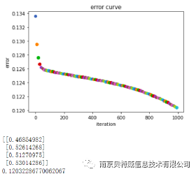
It is not difficult to see that using MSE cannot solve the XOR problem, so what is the reason?

Theoretically it would be possible to use the squared loss function for classification problems as well, but it is not suitable. First, minimizing the squared loss function is essentially equivalent to a maximum likelihood estimate under the assumption that the error follows a Gaussian distribution, whereas most classification problems do not have a Gaussian distribution. Moreover, in practical applications, the cross entropy, in conjunction with the Softmax activation function, can make the larger the loss value, the larger the derivative, and the smaller the loss value, the smaller the derivative, which can speed up the learning rate. However, if the squared loss function is used, the larger the loss, the smaller the derivative, and the learning rate is very slow. Look at the picture below to see the problem.

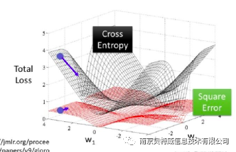
Look at the first result graph above and the third chapter result graph:

If MSE is used as the loss calculation, if the gradient is very small, it is impossible to see whether it is close to the target or far from the target.

Using cross entropy as the loss function, at the beginning, the error will drop significantly. The reason is that the partial derivative of the cross entropy error to the parameter w is very large at the beginning, and the parameter will be updated greatly, so the error will drop faster.

The MSE loss can see that the error changes very gently, which also confirms the above three-dimensional space map, and the error transformation is very slow.

Fourth, the initialization weight problem

1. np's random function

np.random.randn(d0,d1,...,dn): Returns a floating-point number when there is no parameter, returns an array of rank 1 when there is one parameter, and generates an array of the corresponding dimension when there are two or more parameters. The random numbers in it follow a standard normal distribution with a mean of 0 and a standard deviation of 1.

np.random.rand(d0,d1,...,dn) : The parameter function is the same as np.random.randn. The random number is uniformly distributed from 0 to 1, and the random sample value is [0, 1), which cannot be 1.

np.random.randint(low,high,size=None ,dtype= 'l'): low is the minimum value, high is the maximum value, size is the size of the array dimension, dtype is the data type, and the default is np.int. Returns a random integer array, the value range is [low, high), and high cannot be obtained. When high is not filled in, the default random number range is [0, low).

2. Initialize the weights

In order to ensure the difference between input and output, the model can be stable and converge quickly

In order to describe the difference, so think of the variance. Both D(x) and Var(x) represent variance.

The variance formula applied to the product of two random variables:

For forward propagation, only by ensuring that the variances of the activation values of all layers are approximately equal, the information of the training samples passing through the neural network can be kept smooth.

For backpropagation, the gradients of each layer maintain an approximate variance, which also allows the information to flow smoothly in reverse to update the weights.

It is assumed that weights, activations, weighted outputs, network raw outputs and gradients are independent of each other.

Assuming that the activation values and weights are uniformly distributed with mean 0, then the last two terms of the product of the above two random variables are 0.

In order to make the variance of the weighted output z approximately equal to the variance of the activation values in the forward pass, it is recommended to use the tanh() activation function because it has tanh(x) ≈ x at the origin.

Next consider the weighted output of the jth unit of the Lth layer:

In order to make the difference between the sample space and the category space not large, it is to make the variance between them as equal as possible, namely:

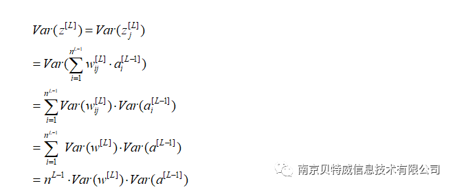
then need

In backpropagation, the same

need

Take the harmonic mean of these two numbers:

(a, b) is the range of initialized weights.

In this example, the number of neurons in the hidden layer is 4, so the weight initialization range can be approximately set to (-1,1).