This may be the most complete set of Python algorithms in history

This article is a collection of Python code for some robotics algorithms (especially auto-navigation algorithms).

Its main features are the following three points: algorithms that are widely used in practice are selected; the dependencies are the least; easy to read and easy to understand the basic idea of ​​each algorithm. Hope it will help you after reading this article.

Table of contents

Python 3.6.x

numpy

scipy

matplotlib

pandas

cvxpy 0.4.x

install the necessary libraries;

Clone this code repository;

Execute the python script in each directory;

If you like it, bookmark this codebase :)

3.1 Extended Kalman Filter Localization

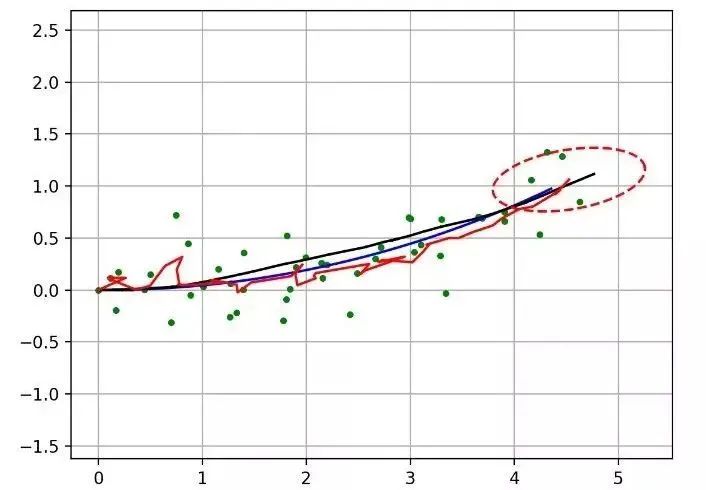
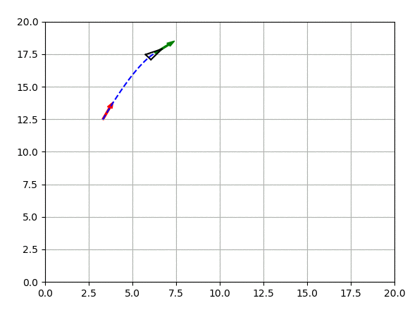
The algorithm utilizes Extended Kalman Filter (EKF) to achieve sensor hybrid localization.

The blue line is the real path, the black line is the dead reckoning trajectory, the green dots are the position observations (such as GPS), and the red line is the path estimated by the EKF.

The red ellipse is the covariance estimated by the EKF.

Related Reading:

Probabilistic Robotics

http://www.probabilistic-robotics.org/

3.2 Lossless Kalman Filter Localization

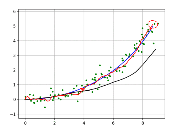
The algorithm utilizes the Unscented Kalman Filter (UKF) to achieve sensor hybrid localization.

Lines and dots have the same meaning as in the EKF simulation example.

Related Reading:

Robot Movement Localization Using Indiscriminately Trained Lossless Kalman Filters

https://www.researchgate.net/publication/267963417_Discriminatively_Trained_Unscented_Kalman_Filter_for_Mobile_Robot_Localization

3.3 Particle filter localization

The algorithm utilizes Particle Filter (PF) to achieve sensor hybrid localization.

The blue line is the real path, the black line is the dead reckoning trajectory, the green dot is the position observation (eg GPS), and the red line is the PF estimated path.

The algorithm assumes that the robot is able to measure the distance to a landmark (RFID).

This measurement is used for PF localization.

Related Reading:

Probabilistic Robotics

http://www.probabilistic-robotics.org/

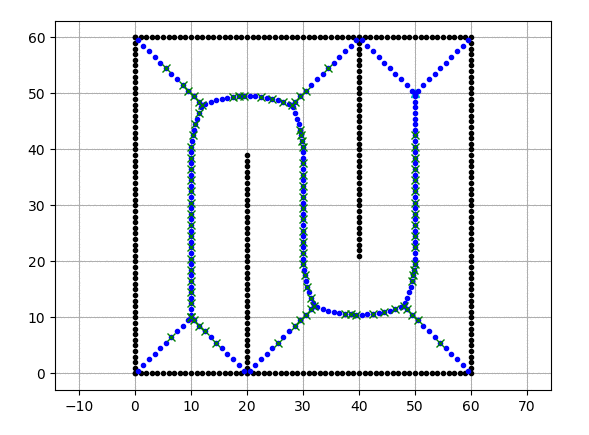
3.4 Histogram filtering localization

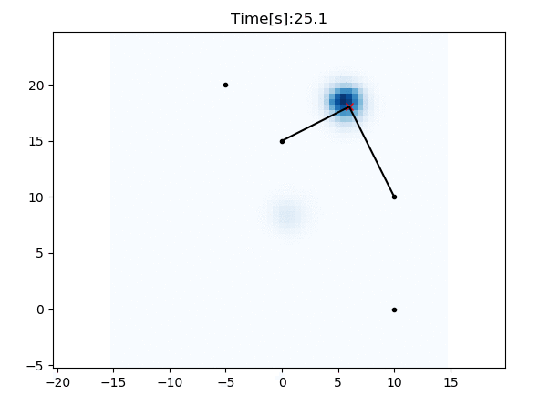
This algorithm is an example of 2D localization using a histogram filter.

The red cross is the actual location and the black dot is the location of the RFID.

The blue boxes are the probability positions of the histogram filter.

In this simulation, x, y are unknowns and yaw is known.

The filter integrates the velocity input and the distance observations obtained from the RFID for localization.

No initial position is required.

Related Reading:

Probabilistic Robotics

http://www.probabilistic-robotics.org/

4.1 Gaussian grid mapping

This algorithm is an example of two-dimensional Gaussian grid mapping.

4.2 Raycasting mesh mapping

This algorithm is an example of a two-dimensional ray casting grid map.

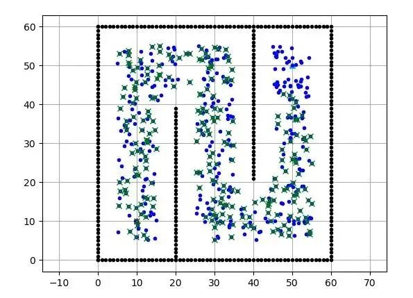
4.3 k-means object clustering

This algorithm is an example of two-dimensional object clustering using the k-means algorithm.

4.4 Shape Recognition of Circular Fitting Objects

This algorithm is an example of object shape recognition using circle fitting.

The blue circle is the actual object shape.

The red cross is the point observed by the distance sensor.

The red circle is the estimated object shape using a circular fit.

An example of Simultaneous Localization and Mapping (SLAM).

5.1 Iterative closest point matching

This algorithm is an example of two-dimensional Iterative Closest Point (ICP) matching using single-value destructuring.

It can calculate rotation and translation matrices from some points to other points.

Related Reading:

Introduction to Robotic Motion: Iterative Closest Point Algorithm

https://cs.gmu.edu/~kosecka/cs685/cs685-icp.pdf

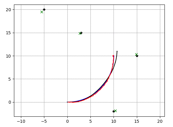
5.2 EKF SLAM

Here is an example of SLAM based on Extended Kalman Filtering.

The blue line is the true path, the black line is the navigation inferred path, and the red line is the path estimated by EKF SLAM.

Green crosses are estimated landmarks.

Related Reading:

Probabilistic Robotics

http://www.probabilistic-robotics.org/

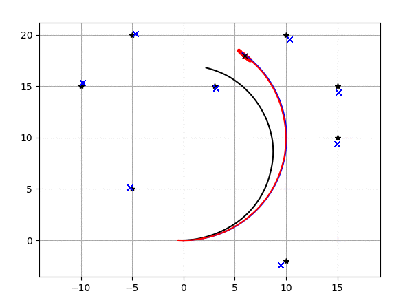
5.3 FastSLAM 1.0

Here is an example of feature-based SLAM with FastSLAM 1.0.

The blue line is the actual path, the black line is the navigation guess, and the red line is the FastSLAM guess.

The red dots are particles in FastSLAM.

The black dots are the landmarks, and the blue crosses are the landmark locations estimated by FastLSAM.

Related Reading:

Probabilistic Robotics

http://www.probabilistic-robotics.org/

5.4 FastSLAM 2.0

Here is an example of feature-based SLAM with FastSLAM 2.0.

The meaning of animation is the same as in the case of FastSLAM 1.0.

Related Reading:

Probabilistic Robotics

http://www.probabilistic-robotics.org/

Tim Bailey's SLAM Simulation

http://www-personal.acfr.usyd.edu.au/tbailey/software/slam_simulations.htm

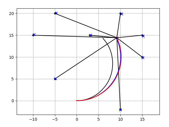
5.5 Graph-based SLAM

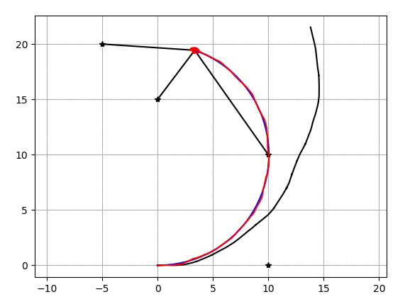
This is an example of graph-based SLAM.

The blue line is the actual path.

The black line is the navigation speculative path.

The red line is the path estimated by the graph-based SLAM.

Black stars are landmarks that are used to generate the edges of the graph.

Related Reading:

Getting Started with Graph-Based SLAM

http://www2.informatik.uni-freiburg.de/~stachnis/pdf/grisetti10titsmag.pdf

6.1 Dynamic window mode

This is a sample code for 2D navigation using Dynamic Window Approach.

Related Reading:

Avoid collisions with dynamic windows

https://www.ri.cmu.edu/pub_files/pub1/fox_dieter_1997_1/fox_dieter_1997_1.pdf

6.2 Grid-based search

Dijkstra's algorithm

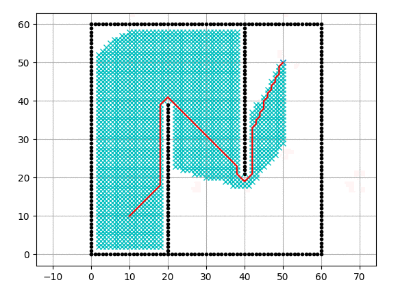
This is a two-dimensional grid-based shortest path planning implemented using Dijkstra's algorithm.

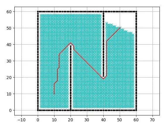
The cyan dots in the animation are the searched nodes.

A* algorithm

The following is the shortest path planning based on two-dimensional grid using the A-star algorithm.

The cyan dots in the animation are the searched nodes.

The heuristic is the two-dimensional Euclidean distance.

Potential Field Algorithm

The following is a two-dimensional grid-based path planning using the potential field algorithm.

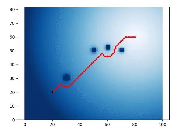
The blue heat map in the animation shows the potential energy of each grid.

Related Reading:

Robot Motion Planning: Potential Energy Function

https://www.cs.cmu.edu/~motionplanning/lecture/Chap4-Potential-Field_howie.pdf

6.3 Model prediction path generation

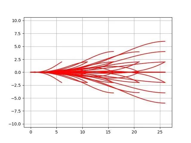
Below is an example of path optimization for model predicted path generation.

The algorithm is used for state lattice planning.

Path Optimization Example

Lookup table generation example

Related Reading:

Optimal Rough Terrain Path Generation for Robots with Wheels

http://journals.sagepub.com/doi/pdf/10.1177/0278364906075328

6.4 State Lattice Planning

This script uses state lattice planning to implement path planning.

This code solves the boundary problem by model predicting path generation.

Related Reading:

Optimal Rough Terrain Path Generation for Robots with Wheels

http://journals.sagepub.com/doi/pdf/10.1177/0278364906075328

State-space sampling of feasible motions for high-performance kinematic robot navigation in complex environments

http://www.frc.ri.cmu.edu/~alonzo/pubs/papers/JFR_08_SS_Sampling.pdf

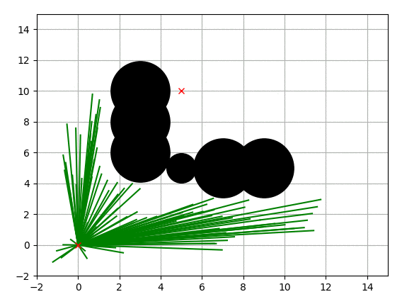
Uniform polar sampling

Biased polar sampling

Lane sampling

6.5 Random Path Graph (PRM) Planning

This Probabilistic Road-Map (PRM) planning algorithm uses Dijkstra's method for graph search.

The blue dots in the animation are the sampling points.

The cyan crosses are the points searched by Dijkstra's method.

The red line is the final path of the PRM.

Related Reading:

random path map

https://en.wikipedia.org/wiki/Probabilistic_roadmap

6.6 Voronoi roadmap planning

This Voronoi Probabilistic Road-Map (PRM) planning algorithm adopts Dijkstra's method on graph search.

The blue dots in the animation are Voronoi points.

The cyan crosses are the points searched by Dijkstra's method.

The red line is the final path of the Voronoi path map.

Related Reading:

Robot motion planning

https://www.cs.cmu.edu/~motionplanning/lecture/Chap5-RoadMap-Methods_howie.pdf

6.7 Rapid Search Random Tree (RRT)

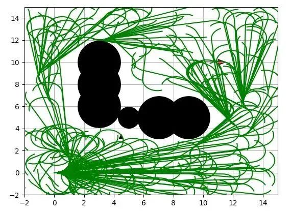
Basic RRT

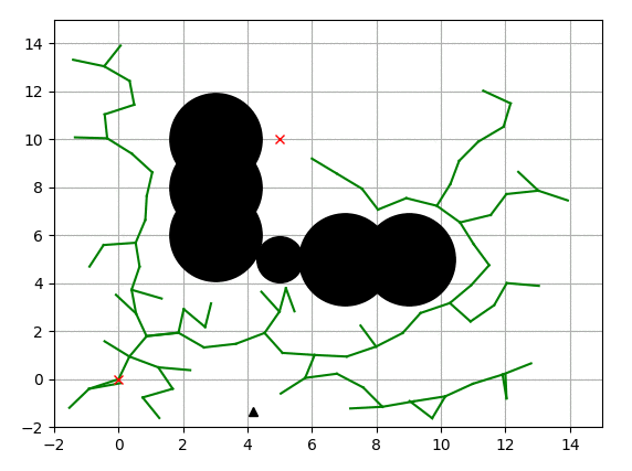
This is a simple path planning code using Rapidly-Exploring Random Trees (RRT).

The black circle is the obstacle, the green line is the search tree, and the red cross is the starting position and the target position.

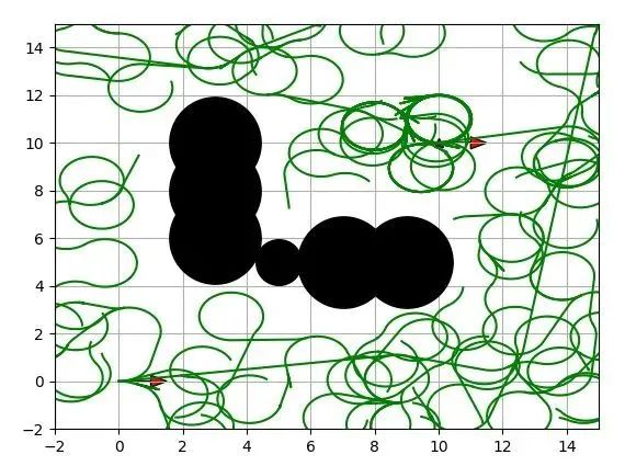
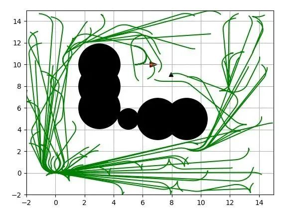
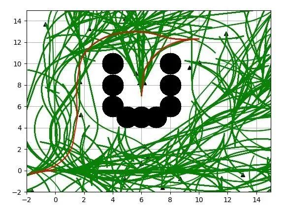
RRT*

Here is the path planning code using RRT*.

The black circle is the obstacle, the green line is the search tree, and the red cross is the starting position and the target position.

Related Reading:

Incremental sampling based algorithm for optimal motion planning

https://arxiv.org/abs/1005.0416

Sampling-Based Algorithms for Optimal Motion Planning

http://citeseerx.ist.psu.edu/viewdoc/download?doi=10.1.1.419.5503&rep=rep1&type=pdf

基于Dubins路径的RRT

为汽车形机器人提供的使用RRT和dubins路径规划的路径规划算法。

基于Dubins路径的RRT*

为汽车形机器人提供的使用RRT*和dubins路径规划的路径规划算法。

基于reeds-shepp路径的RRT*

为汽车形机器人提供的使用RRT*和reeds shepp路径规划的路径规划算法。

Informed RRT*

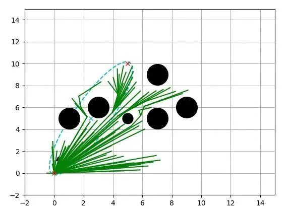
这是使用Informed RRT*的路径规划代码。

青色椭圆为Informed RRT*的启发采样域。

相关阅读：

Informed RRT*：通过对可接受的椭球启发的直接采样实现最优的基于采样的路径规划

https://arxiv.org/pdf/1404.2334.pdf

批量Informed RRT*

这是使用批量Informed RRT*的路径规划代码。

相关阅读：

批量Informed树（BIT*）：通过对隐含随机几何图形进行启发式搜索实现基于采样的最优规划

https://arxiv.org/abs/1405.5848

闭合回路RRT*

使用闭合回路RRT*（Closed loop RRT*）实现的基于车辆模型的路径规划。

这段代码里，转向控制用的是纯追迹算法（pure-pursuit algorithm）。

速度控制采用了PID。

相关阅读：

使用闭合回路预测在复杂环境内实现运动规划

http://acl.mit.edu/papers/KuwataGNC08.pdf）

应用于自动城市驾驶的实时运动规划

http://acl.mit.edu/papers/KuwataTCST09.pdf

[1601.06326]采用闭合回路预测实现最优运动规划的基于采样的算法

https://arxiv.org/abs/1601.06326

LQR-RRT*

这是个使用LQR-RRT*的路径规划模拟。

LQR局部规划采用了双重积分运动模型。

相关阅读：

LQR-RRT*：使用自动推导扩展启发实现最优基于采样的运动规划

http://lis.csail.mit.edu/pubs/perez-icra12.pdf

MahanFathi/LQR-RRTstar：LQR-RRT*方法用于单摆相位中的随机运动规划

https://github.com/MahanFathi/LQR-RRTstar

6.8 三次样条规划

这是段三次路径规划的示例代码。

这段代码根据x-y的路点，利用三次样条生成一段曲率连续的路径。

每个点的指向角度也可以用解析的方式计算。

6.9 B样条规划

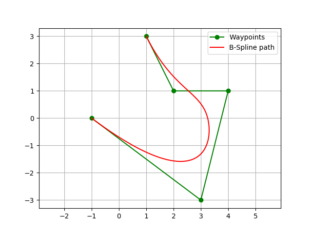
这是段使用B样条曲线进行规划的例子。

输入路点，它会利用B样条生成光滑的路径。

第一个和最后一个路点位于最后的路径上。

相关阅读：

B样条

https://en.wikipedia.org/wiki/B-spline

6.10 Eta^3样条路径规划

这是使用Eta ^ 3样条曲线的路径规划。

相关阅读：

eta^3-Splines for the Smooth Path Generation of Wheeled Mobile Robots

https://ieeexplore.ieee.org/document/4339545/

6.11 贝济埃路径规划

贝济埃路径规划的示例代码。

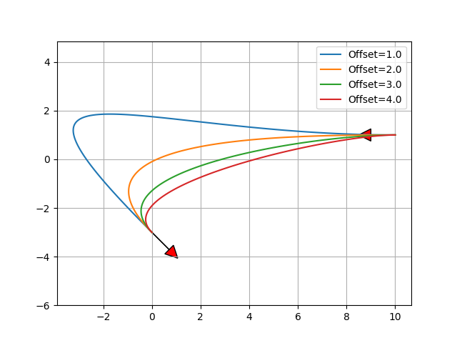
根据四个控制点生成贝济埃路径。

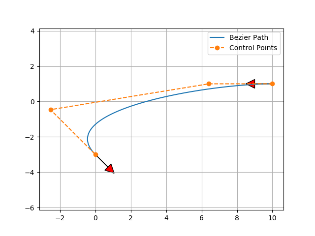
改变起点和终点的偏移距离，可以生成不同的贝济埃路径：

相关阅读：

根据贝济埃曲线为自动驾驶汽车生成曲率连续的路径

http://citeseerx.ist.psu.edu/viewdoc/download?doi=10.1.1.294.6438&rep=rep1&type=pdf

6.12 五次多项式规划

利用五次多项式进行路径规划。

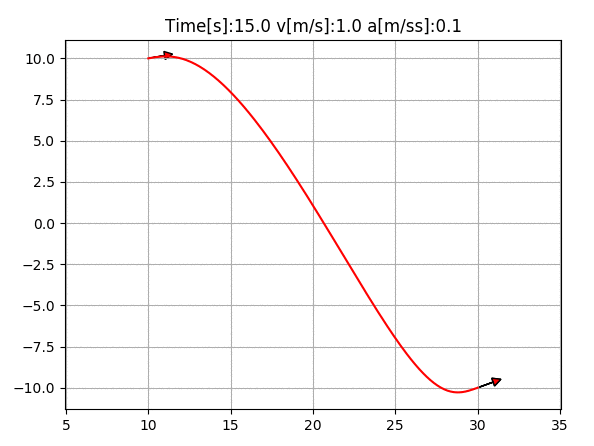
它能根据五次多项式计算二维路径、速度和加速度。

相关阅读：

用于Agv In定位的局部路径规划和运动控制

http://ieeexplore.ieee.org/document/637936/

6.13 Dubins路径规划

Dubins路径规划的示例代码。

相关阅读：

Dubins路径

https://en.wikipedia.org/wiki/Dubins_path

6.14 Reeds Shepp路径规划

Reeds Shepp路径规划的示例代码。

相关阅读：

15.3.2 Reeds-Shepp曲线

http://planning.cs.uiuc.edu/node822.html

用于能前进和后退的汽车的最优路径

https://pdfs.semanticscholar.org/932e/c495b1d0018fd59dee12a0bf74434fac7af4.pdf

ghliu/pyReedsShepp：实现Reeds Shepp曲线

https://github.com/ghliu/pyReedsShepp

6.15 基于LQR的路径规划

为双重积分模型使用基于LQR的路径规划的示例代码。

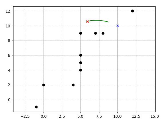
6.16 Frenet Frame中的最优路径

这段代码在Frenet Frame中生成最优路径。

青色线为目标路径，黑色叉为障碍物。

红色线为预测的路径。

相关阅读：

Frenet Frame中的动态接到场景中的最优路径生成

https://www.researchgate.net/profile/Moritz_Werling/publication/224156269_Optimal_Trajectory_Generation_for_Dynamic_Street_Scenarios_in_a_Frenet_Frame/links/54f749df0cf210398e9277af.pdf

Frenet Frame中的动态接到场景中的最优路径生成

https://www.youtube.com/watch?v=Cj6tAQe7UCY

7.1 姿势控制跟踪

这是姿势控制跟踪的模拟。

相关阅读：

Robotics, Vision and Control - Fundamental Algorithms In MATLAB® Second, Completely Revised, Extended And Updated Edition | Peter Corke | Springer

https://www.springer.com/us/book/9783319544120

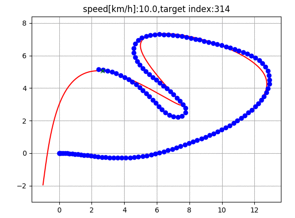
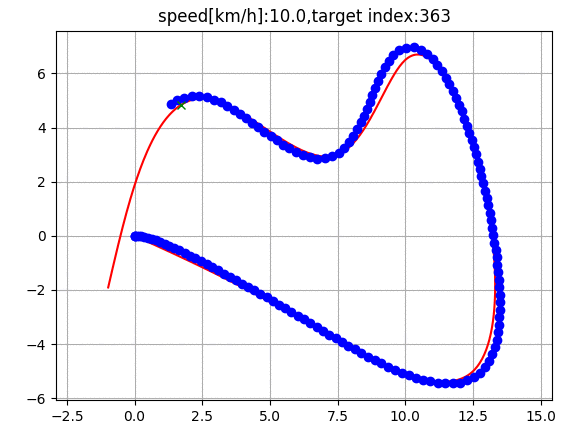
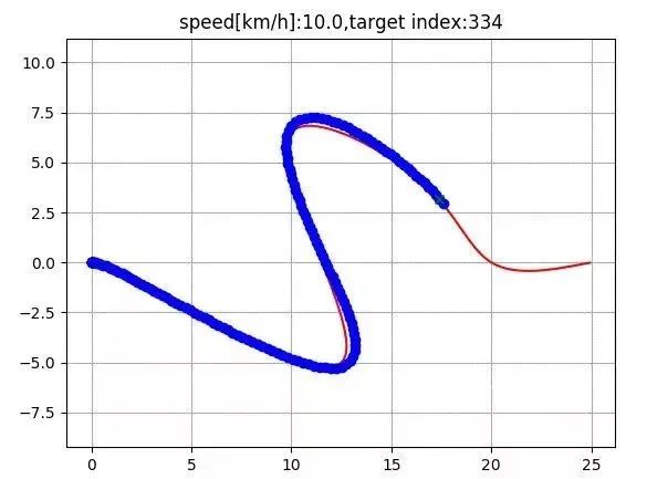
7.2 纯追迹跟踪

使用纯追迹（pure pursuit）转向控制和PID速度控制的路径跟踪模拟。

红线为目标路线，绿叉为纯追迹控制的目标点，蓝线为跟踪路线。

相关阅读：

城市中的自动驾驶汽车的运动规划和控制技术的调查

https://arxiv.org/abs/1604.07446

7.3 史坦利控制

使用史坦利（Stanley）转向控制和PID速度控制的路径跟踪模拟。

相关阅读：

史坦利：赢得DARPA大奖赛的机器人

http://robots.stanford.edu/papers/thrun.stanley05.pdf

用于自动驾驶机动车路径跟踪的自动转向方法

https://www.ri.cmu.edu/pub_files/2009/2/Automatic_Steering_Methods_for_Autonomous_Automobile_Path_Tracking.pdf

7.4 后轮反馈控制

利用后轮反馈转向控制和PID速度控制的路径跟踪模拟。

相关阅读：

城市中的自动驾驶汽车的运动规划和控制技术的调查

https://arxiv.org/abs/1604.07446

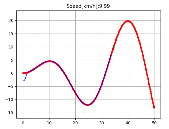
7.5 线性二次regulator（LQR）转向控制

使用LQR转向控制和PID速度控制的路径跟踪模拟。

相关阅读：

ApolloAuto/apollo：开源自动驾驶平台

https://github.com/ApolloAuto/apollo

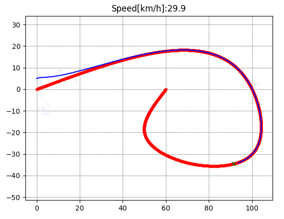
7.6 线性二次regulator（LQR）转向和速度控制

使用LQR转向和速度控制的路径跟踪模拟。

相关阅读：

完全自动驾驶：系统和算法 - IEEE会议出版物

http://ieeexplore.ieee.org/document/5940562/

7.7 模型预测速度和转向控制

使用迭代线性模型预测转向和速度控制的路径跟踪模拟。

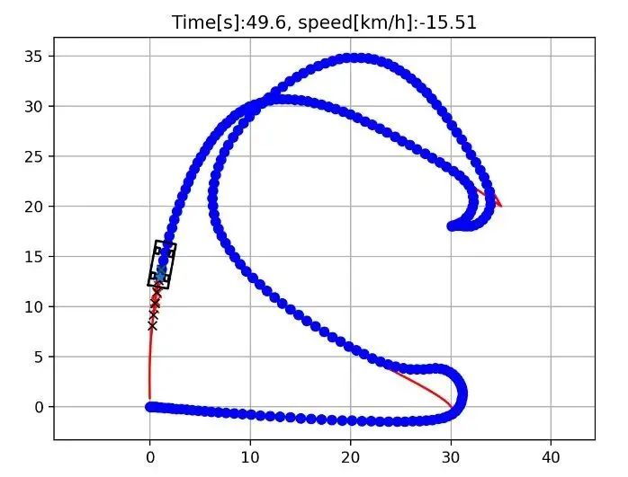
这段代码使用了cxvxpy作为最优建模工具。

车辆动态和控制 | Rajesh Rajamani | Springer

http://www.springer.com/us/book/9781461414322

MPC课程资料 - MPC Lab @ UC-Berkeley

http://www.mpc.berkeley.edu/mpc-course-material

八、项目支持

可以通过Patreon（
https://www.patreon.com/myenigma）对该项目进行经济支持。

如果你在Patreon上支持该项目，则可以得到关于本项目代码的邮件技术支持。

本文作者包括有Atsushi Sakai (@Atsushi_twi)，Daniel Ingram，Joe Dinius，Karan Chawla，Antonin RAFFIN，Alexis Paques。

项目地址：
https://github.com/AtsushiSakai/PythonRobotics

版权归原作者所有，如有侵权，请联系删除。

【海豚人工智能与大数据实验室】是“一站式”大数据分析及人工智能的教育实训+科研平台,  由北美海归团队创立的杭州睿数科技有限公司自主研发。通过“沉浸式” “交互式”的在线虚拟实验平台,结合丰富的真实行业案例和数据集，切实解决大数据及人工智能教育培训环节的痛点。通过我们的整体解决方案，实现 “大数据 + X”，“人工智能 + X”的跨专业、跨学科复合型人才培养。全面助力中国人工智能，大数据产业的快速发展！

欢迎全国高校、培训机构、渠道合作伙伴与我们联系，开展合作！

联系热线：400-001-3538 或 137-5084-3241

联系邮箱：[email protected]