introduction
The intuitive judgment of the correlation between variables is usually carried out by observing the variable scatter plot, and the mathematical judgment is judged by the covariance formula; the degree of the correlation between the variables is judged by the three major correlation coefficients in statistics. Under different conditions, different correlation coefficients apply.
import numpy as np
import pandas as pd
import matplotlib.pyplot as plt#一次性导入需要的包
read data
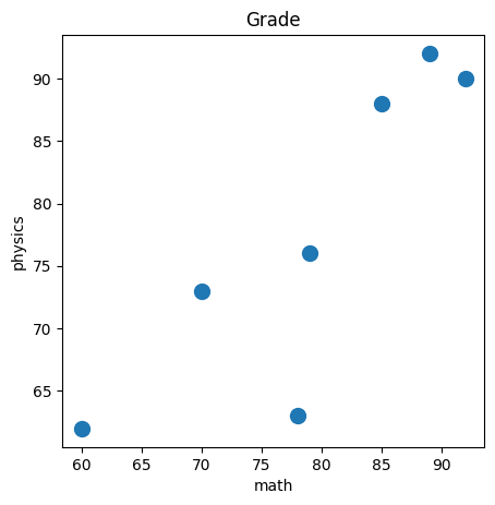
math = [89,78,79,85,92,70,60]#math 成绩,生成一个list
physics = [92,63,76,88,90,73,62]#physics 成绩,生成一个list
grade = {'math':math,'physics':physics}#根据成绩,生成一个字典
data = pd.DataFrame(grade)#根据字典,生成一个dataframe,方便后面调用pandas的函数
draw a scatter plot
plt.figure(figsize=(5, 5), dpi=100) #画布设置,可设置参数。画布可以不设置。

plt.scatter(math, physics,s=100)  # 第一个参数为横轴。第二个参数为纵轴。 第三个参数为圆点大小,可选参数
#plt.scatter(math, physics,s=100,c='red',alpha=0.5) #红色圆点,半透明,scatter还有其他很多可选参数。感兴趣可以自行查阅官方文档或者相关资料进行学习

plt.xlabel('math')#横轴标签
plt.ylabel('physics')#纵轴标签

plt.title("Grade")#图题

plt.show()
Covariance
#np.cov(math,physics)# 输出协方差矩阵

# np.cov(x,y)[0][0] #向量x的样本方差
# np.cov(x,y)[0][1] #向量x与y的协方差
# np.cov(x,y)[1][1] #向量y的样本方差

#data['math'].cov(data['physics'])#输出协方差值
data.cov()#输出协方差矩阵
| math | physics | |
|---|---|---|
| math | 124.666667 | 120.000000 |
| physics | 120.000000 | 158.238095 |
Pearson coefficient
data.corr()
#data.corr("pearson")#默认method 是"pearson",可以指定为“spearman”或者“kendall”
| math | physics | |
|---|---|---|
| math | 1.000000 | 0.854379 |
| physics | 0.854379 | 1.000000 |
Spearman coefficient
data.corr("spearman")
| math | physics | |
|---|---|---|
| math | 1.000000 | 0.928571 |
| physics | 0.928571 | 1.000000 |
From here, we can actually see that the spearman coefficient is tolerant of outliers. The calculated value is larger than Pearson's value and reflects stronger data correlation.
data.corr("kendall")
| math | physics | |
|---|---|---|
| math | 1.000000 | 0.809524 |
| physics | 0.809524 | 1.000000 |