4 Ways to Display Negative Numbers in Red in Excel

Hello everyone, I'm Uncle Xia, a 10-year-old driver in the workplace. I'm currently an engineer in a Fortune 500 company. I use Excel all the year round at work.

【Previous Article 】A Complete Guide to Drop-Down Lists

What I want to share with you today is how to display negative numbers as red in Excel. Uncle Xia summed up the following four methods for you.

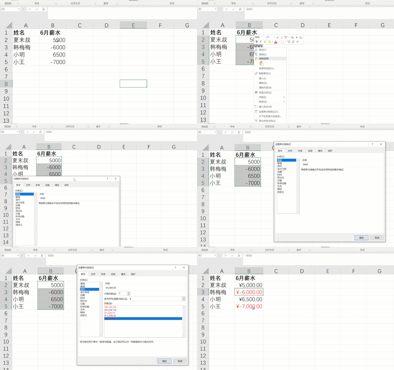
Method 1: Use Number Format

The most direct way is to use the number format or currency format, the steps are as follows:

selected range of cells
Right-click and select "Format Cells"
Select "Number" - "Currency" in turn, then select the last negative form, and click "OK"

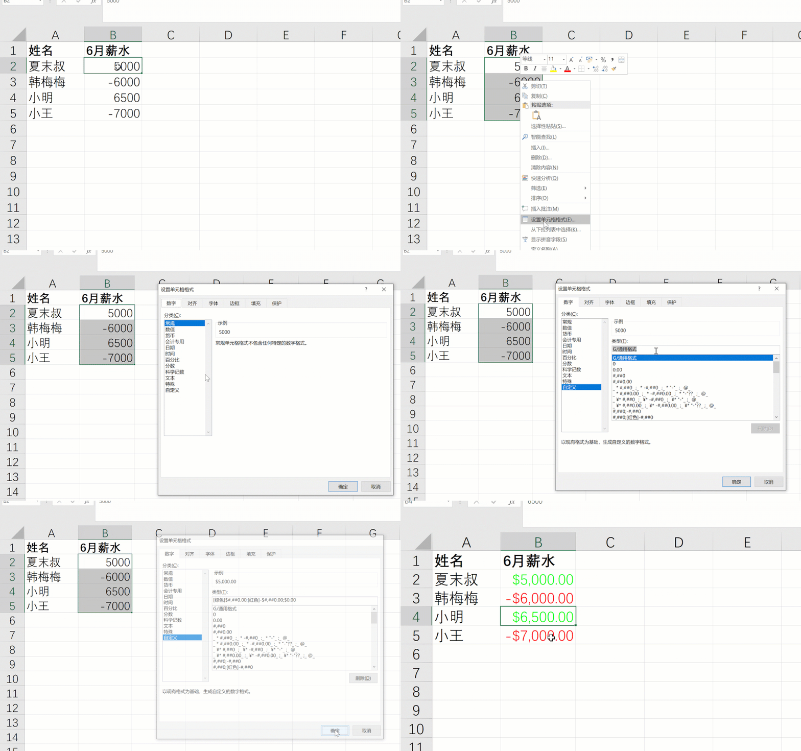
‍Method 2: Use a custom format

We can also set it by customizing the format, such as displaying positive numbers in green and negative numbers in red. Proceed as follows:

selected range of cells
Right-click and select "Format Cells"
Select "Number" - "Custom"
Enter this code in the "Type" input box: [green]$#,##0.00;[red]-$#,##0.00;$0.00
Finally click "OK"

‍

Let's analyze what this code means.

This code consists of multiple parts:

① Positive, negative and zero values are separated by semicolons

② The positive number is in the first position, we can specify a color in the square brackets in front of the number format string, such as green

③ The negative number is in the second position, you can also specify a color

④ The zero value is in the third position, and a color can also be specified

Method 3: Use Conditional Formatting

Conditional formatting can format cells based on custom rules, and can modify any type of cell formatting, such as borders, font sizes, font styles, and fill colors. You can also change the font color to red when the value of the cell is less than 0.

The operation steps are as follows:

First select the cell range, then click Start - Conditional Formatting - New Rule
Select "Format only cells that contain"
Select the cell value in turn - less than, enter 0 in the input box on the right
Then click [Format] - [Font], select red, and click OK.

‍Method 4: Use VBA code

We can also automate the processing by writing VBA code. Press the shortcut key Alt + F11 to open the VBA code editor, click "Insert" - "Module" at the top, and you can add VBA code and save it in a new window.

Sub ChangeFontColor()Dim rng As Range
For Each rng In Selection    If rng.Value < 0 Then        rng.Font.Color = vbRed    Else        rng.Font.Color = vbBlack    End IfNext rngEnd Sub

This code will loop in the selected area of the worksheet to check whether the value of the cell is less than 0, if it is less than 0, set the color to red; otherwise, set the color to black.

Specific steps are as follows:

Select the area with numbers
Press the shortcut key Alt + F8 to pop up the "Macro" dialog box
Select ChangeFontColor and click "Execute" directly

Well, I'll share it here with you today. If you like Uncle Xia's article, remember to like and watch Uncle Xia, thank you~~

[Recommendation of previous articles]